Reduction

This guide assumes that you have got started with the HiPERCAM pipeline (see At the telescope for a quick start to observing), but now would like a more detailed guide to reducing your data. It covers the following steps:

Bias correction

CCD images come with a near-constant electronic offset called the “bias” which ensures that the counts are always positive and helps ensure optimum readout properties. This offset does not represent genuine detected light and must be subtracted off any image. The standard approach is to take a set of zero illumination frames quickly to avoid the build-up of counts either from light leakage or thermal noise.

Bias frames can be quickly taken with HiPERCAM, ULTRACAM and ULTRASPEC. All dome lights should be off, the focal plane slide should be in to block light, and ideally the telescope mirrors closed (in the case of ULTRASPEC point the M4 mirror towards the 4k camera). You may also want to put a low transmission filter in. Bias frames should be taken with clears enabled if possible and with the shortest possible exposure delay (hit “page down” in the camera driver gui) to minimise the time spent accumulating photons.

We standardly take 51 or 101 bias exposures, more for small formats. These can be combined by averaging pixel-by-pixel with rejection of outliers to remove cosmic rays, or by taking the pixel-by-pixel median. These operations can be carried out with combine once individual exposures have been extracted with grab. It is always advisable to inspect the frames visually with rtplot to check for problems, e.g. with the readout, or light getting onto the images. So long as several tens of bias exposures are available, then clipped mean combination of frames is preferable to median combination because it leads to a lower level statistical noise. Median combination works better for small number of frames where the clipped mean can be less effective at removing outliers. Usually one should combine bias frames with offsets to correct for any drift in the mean level which could otherwise affect the action of combine.

The two operations of grab followed by combine, along with clean-up of the temporary files can be carried out with the single command makebias. This also saves the frames to a temporary location to avoid polluting the working directory with lots of files. Thus assuming all frames in bias run run0002 are OK, the following command will make the combined bias frame:

makebias run0002 1 0 3.0 yes run0002

rejecting pixels deviating by more that 3.0 sigma from the mean. You might also want to create a more memorable name as a soft link to the output hcm file, depending upon the particular type of bias:

ln -s run0002.hcm bias1x1_ff_slow.hcm

for example, for a 1x1 binned, full-frame bias in slow readout mode. I like this approach because one can quickly see (e.g. ‘ls -l’) which run a given calibration frame came from.

Once you have a bias frame, then it can be used by editing in its name in the calibration section of the reduce file.

Note

One should take bias calibration images in all the output formats used to guard against small changes that can occur as one changes output window formats. We have not yet established the significance of this for HiPERCAM.

Warning

For HiPERCAM, do not take bias frames too soon after (within less than 20 minutes) powering on the CCDs to avoid higher than normal dark current. makebias include a plot option to check this. Make sure to look at this if the bias is taken not long after a power on. ULTRA(CAM|SPEC) are better behaved in this respect, but it is always worth plotting the mean levels which ideally should drift by at most a few counts.

Dark correction (thermal noise)

If a CCD is left exposing in complete darkness, counts accumulate through thermal excitation known as “dark current”. Correction for this is particularly important for long exposure images. Both HiPERCAM and ULTRASPEC are kept quite cold and have relatively little dark current, so it is often safe to ignore it. It is also very often not at all easy to take dark calibration frames because of light leakage. At minimum they typically need to be taken at night with the dome closed, so they are a good bad weather calibration. One should normally take a set of biases before and after as well to allow for bias level drift. Dark current is however important for ULTRACAM where the CCDs run relatively warm. In particular there are multiple “hot pixels” with dark currents significantly above the background. Figure Fig. 1 shows histograms of the combination of a series of 60-second darks. 600 on the X-axis corresponds to 10 counts/second, and there are some pixels over 10x higher than this.

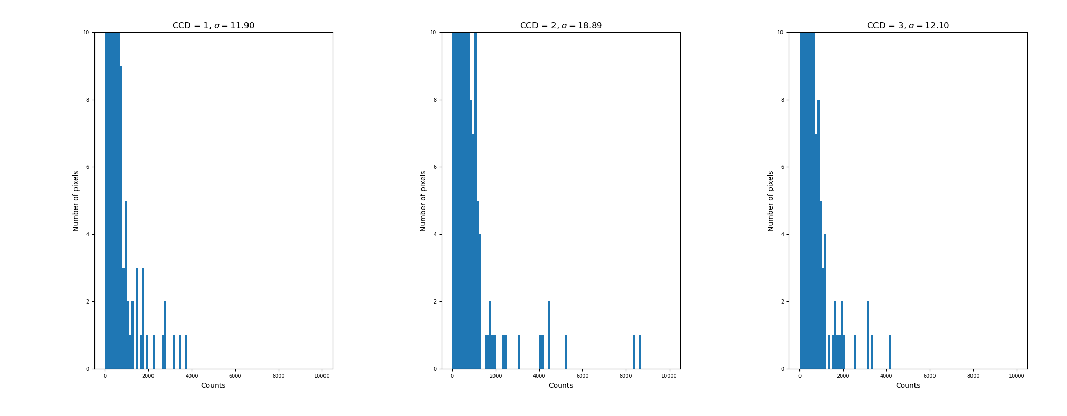
Fig. 1 Histogram of an ULTRACAM dark frame showing that there are a few pixels that rack up thermal counts at over 100 per second.

The program makedark handles making dark calibration frames including correction for whatever exposure is included in the bias. If dark current is significant, then the flat fields should also be corrected. Note that correcting for dark current does not mean that you should not try to avoid hot pixels; the worst of these could add significant noise and the very worst are poorly behaved and do not correct well, but certainly dark correction should offset the worst effects of thermal noise. The effect of hot pixels is particularly important in the u-band of ULTRACAM where count rates from targets are generally lower. If you plot a defect file which include hot pixels with rtplot or nrtplot, any marked hot pixels will appear as integers with their count rate in counts per second. If you zoom in close around targets of interest, it will be obvious whether you need to move the position.

Warning

makedark uses clipped mean combination, which is rather insensitive for small numbers of points, so ideally you need at least 20+ frames, or to take some care with the value of sigma that you set. This is a crucial step to avoid propagating cosmic rays into the final output.

Flat field correction

CCDs are not of uniform sensitivity. There are pixel-to-pixel variations, there may be dust on the optics, and there may be overall vigetting which typically causes a fall in sensitivity at the edge of the field. These are all reasons while observing to keep your targets as fixed in position as possible. However, in addition, it helps to try to correct for such variations. To account for this the standard approach is to take images of the twilight sky just after sunset or before sunrise. Best of all if the sky is free of many stars, but in any case one should always offset the (multiple) sky field frames taken so that stars can be medianed out of the flat field. Normally we move in a spiral pattern to accomplish this, so you will usually see a comment about “telescope spiralling” and should look for moving objects in flat fields. If things move, that is good.

At the GTC, HiPERCAM’s driving routine, hdriver can drive the telescope as well as the instrument, making spiralling during sky flats straightforward. One can normally acquire more than 100 frames in a single run, but the different CCDs will have different count levels on any one frame, and will come out of saturation at different times. The count levels will also be falling or rising according to whether the flats were taken at evening or morning twilight. At the NTT and TNT, we ask the TO to spiral the telescope.

The task of making the flat fields is to combine a series of frames with differing count levels, while removing features that vary between images (cosmic rays). In order to do this, one must normalise the images by their mean levels, but weight them appropriately in the final combination to avoid giving too much weight to under-exposed images. This is tedious by hand, and therefore the command makeflat was written to carry out all the necessary tasks.

As with the biases, it is strongly recommended that you inspect the frames to be combined using rtplot to avoid including any disastrous ones. Saturated frames can be spotted using user-defined mean levels at which to reject frames. The documentation of makeflat has details of how it works, and you are referred to this for more information. Recommended mean level limits are ~4000 for each CCD for the lower limits, and (55000, 58000, 58000, 50000 and 42000) for CCDs 1 to 5 (HiPERCAM), (50000, 28000 and 28000) for ULTRACAM and 50000 for ULTRASPEC. The low upper level for CCD 5 of HiPERCAM is to avoid a nasty feature that develops in the lower-right readout channel at high count levels. The limits for ULTRACAM are to stop “peppering” whereby charge transfers between neighbouring pixels in the green and blue CCDs especially.

Warning

It is highly advisable to compute multiple versions of the flat field using different values of the parameter ngroup which can have a significant effect on the removal of stars from the final frame and then to compare the results against each other. See makeflat.

Defringing

With HiPERCAM there is significant fringing in the z-band. ULTRACAM shows it is the z-band and to a much lesser extent in the i-band. Fringing does not flat-field away because it is the result of illumination by the emission-line dominated night sky whereas twilight flats come from broad-band illumination.

De-fringing in the pipeline works by comparing differences across many pairs of points in the data versus a reference “fringe map”. The pairs of points should lie on peaks and troughs of the fringes. Figure Fig. 2 shows fringes from HiPERCAM’s z-band arm.

Fig. 2 Fringe map of HiPERCAM z-band CCD with peak/trough pairs, created from dithered data taken on 2018-04-15 on the GTC.

The idea is to estimate the ratio of fringing amplitude in the data versus the reference image. The effect of defringing can be seen by applying it in nrtplot, and grab. The latter has a “verbose” option which prints out data that might help when setting up for reduction where there are two editing parameters rmin and rmax that are tricky to get a feel for.

There are two scripts specific to fringing in the pipeline called makefringe and setfringe. makefringe builds a fringe map from dithered data; you may be best off just using a pre-prepared frame unless you have specifically acquired such data. setfringe defines peak/trough pairs, and again you may be able to use a pre-prepared file, although for specially window formats it may make sense to adapt the standard set of pairs. See Useful files for pre-prepared files.

Bad pixels and defect files

There is no explicit accounting for bad pixels in the pipeline (yet). The approach has always been to try to avoid them in the first place. We do so through plotting of files of defects during acqusition. See Useful files for pre-prepared files.

Aperture files

The pipeline photometry provides straightforward aperture photometry. Many of the details can be defined when setting the apertures using setaper. Not only can you choose your targets, but you can mask nearby stars from the sky aperture, and you can to a certain extent sculpt your target apertures which can help with blended interlopers by including them in an over-sized aperture.

A key decision to be made at this stage is whether you think your target will remain detectable on each frame throughout the run. Detectable means that it’s position can be measured and thus the relevant aperture re-positioned. If not, then setaper gives you the option of linking any target to another, with the idea that a brighter target can define the position shifts which are applied to the fainter target. Linking is best reserved for the most difficult cases because it does bring its own issues: see the sections on linked apertures and aperture positioning for more details.

An example of a set of apertures showing all these features is shown in Fig. 3.

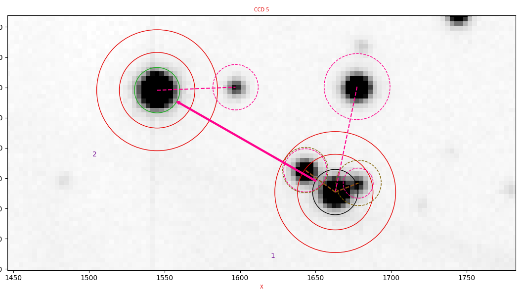
Fig. 3 Example of a complex set of apertures. The target is at the centre of the circles in the lower-right. The comparison star is in the upper-left. [click on the image to enlarge it].

In this case the target star has two nearby companions which causes three problems: (1) the sky annulus may include flux from the companions, (2) the target aperture can include a variable contribution from the companions, depending upon the seeing, and (3) it is hard to locate the object because the position location can jump to the nearby objects. The set of apertures shown in Fig. 3 combats these problems as follows. First, there are pink/purplish dashed circles connected to the centre of the apertures. These are mask regions which exclude the circled regions from any consideration in sky estimation. NB they do not exclude the pixels from inclusion in target apertures; this is not possible without systematic bias without full-blown profile fits. Second, are somewhat similar brown/green dashed circles. These are extra apertures which indicate that the flux in the regions enclosed is to be added to the flux in the target aperture. This offsets the problem of variable amounts of nearby stars’ flux being included in the aperture. Finally, the thick pink arrow pointing from the lower-right (target) aperture to the upper-left reference aperture (green circle) links the target aperture. This means its position is calculated using a fixed offset from the reference aperture. This is often useful for very faint targets, or those, which like the one shown here, have close-by objects that can confuse the re-positioning code. See the sections on linked apertures and aperture positioning for more details.

Reduction files

Once you have defined the apertures for all CCDs that you can, you can create a reduction file using genred. This reads which CCDs and apertures have been set and tries to create a file that at will work with reduce, even if it may well not be ideal. Once you have this file, then you should expect to go through a sequence of running reduce, adjusting the reduce file, re-running reduce until you have a useful plot going. As mentioned above, it is inside the reduce file that you can set the name of your bias, and also the flat field file. You should experiment with changing settings such as the extraction lines and aperture re-position section to get a feel for the different parameters.

The two keys elements to get right in the reduction files are the sections concerning how the apertures are re-located and the extraction. The former is the trickier one. The apertures are re-located in a two-step process. First a search is made in a square box centred on the last position measured for a set of “reference” targets (if they have been defined). The size of this box (search_half_width) is important. If it is too small, your targets may jump beyond it and the reduction is likely to fail as that will set an error condition from which it may never recover. On the other hand, too large, and you could jump to a nearby object, and you also increase the chance of cosmic rays causing problems even though the search uses gaussian smoothing to reduce their influence. The main way to combat this is to choose bright, well-isolated stars as reference target. The shifts from the reference targets are used to place the profile fit boxes and avoid the need to searches over non-reference targets. This can be a great help on faint targets. The main decision on extraction is whether to use variable or fixed apertures (I usually recommend variable), optimal or normal extraction (I usually recommend normal), and the various aperture radii. It is recommended to plot the images in reduce at least once, zoomed in on your target to get a feel for this. Depending on circumstances, significant improvements to the photometry can be made with careful choices on these parameters; do not assume that the file produced by genred is in any way the last word; there is no automatic way to come up with the ideal choices which depend upon the nature of the field and conditions.

Plotting results

reduce delivers a basic view of your data as it comes in, which is usually enough at the telescope. If you want to look at particular features, then you should investigate the command plog. This allows you to plot one parameter versus another, including division by comparison stars. If you use Python, the plog code is a good place to start from when analysing your data in more detail. In particular it shows you how to load in the rather human-unreadable HiPERCAM log files (huge numbers of columns and rows). While observing plog is helpful for plotting the sky level as twilight approaches.

Customisation

You may well find that your data has particular features that the current pipeline does not allow for. An obvious one is with crowded fields, which can only roughly be accommodated with judicious application of the options within setaper. The pipeline does not aim to replicate packages designed to handle crowded fields, and you are best advised to port the data over into single frames using grab, remembering that the ‘hcm’ files are nothing more than a particular form of FITS. If your data requires only a small level of tweaking then there are a few simple aritematical commands such as add and cmul that might help, but it is not the intention to provide a full suite of tools that can deal with all cases. Instead, the recommended route is to code Python scripts to manipulate your data, and the The API is designed to make it relatively easy to access HiPERCAM data. If you devise routines of generic interest, you are encouraged to submit them for possible inclusion within the main pipeline commands. The existing pipeline commands are a good place to start when looking for examples.

The reduce log files

reduce writes all results to an ASCII log file. This can be pretty enormous with many entries per line. The log file is self-documenting with an extensive header section which is worth a look through. In particular the columns are named and given data types to aid ingestion into numpy recarrays. The pipeline command plog provides a crude interface to plotting these files, and module hipercam.hlog should allow you to develop scripts to access the data and to make your own plots. hlog2fits can convert the ASCII logs into a more comprehensible FITS versions, with one HDU per CCD. These can be easily explored with standard FITS utilities like fv. Note however that the ASCII logs comes with a lot of header lines that FITS is singularly bad for, so the ASCII logs are to be preferred in the main. They are also the ones expected for the flagcloud script which allows you to interactively define cloudy and junk data. Here is a short bit of code to show you how you might plot your data, assuming you had the pipeline available:

# import matplotlib
import matplotlib.pyplot as plt

# import the pipeline
import hipercam as hcam

# load the reduction log. Creates
# a hipercam.hlog.Hlog object
hlg = hcam.hlog.Hlog.rascii('run0012.log')

# Extract a hipercam.hlog.Tseries from
# aperture '1' from CCD '2'
targ = hlg.tseries('2','1')

# now the comparison (aperture '2')
comp = hlg.tseries('2','2')

# take their ratio (propagates uncertainties correctly)
lc = targ / comp

# Make an interactive plot
lc.mplot(plt)
plt.show()

The methods of hipercam.hlog.Tseries are worth looking through. e.g. you can convert to magnitudes, change the time axis, dump to an ASCII file, etc.

ULTRA(CAM|SPEC) vs HiPERCAM

The HiPERCAM pipeline is designed to be usable with ULTRA(CAM|SPEC) data as well as data from HiPERCAM itself. You will need a different set of CCD defects, otherwise the two are very similar. One extra ULTRACAM needs is proper dark subtraction (see above), while the z-band (CCD 5) images from HiPERCAM need fringe correction (as do z-band from ULTRA(CAM|SPEC) but it is much rarer). Finally, at the telescope you can access the ULTRA(CAM|SPEC) file server using uls versus hls for HiPERCAM, and you will need the environment variable ULTRACAM_DEFAULT_URL to have been set (standard on the “observer” accounts at the TNT and NTT).

Trouble shooting reduction

There are several things you can do to avoid problems during reduction. The main thing to avoid is that reduce loses your target or the comparison stars.

Aperture positioning

Tracking multiple targets in multiple CCDs over potentially tens of thousands of frames can be a considerable challenge. A single meteor or cosmic ray can throw the position of a target off and you may never recover. This could happen after many minutes of reduction have gone by, which can be annoying. It is by far the most likely problem that you will encounter, because once the aperture positions are determined, extraction is trivial. The ‘apertures’ section of reduce files has multiple parameters designed to help avoid such problems.

As emphasised above, if you identify a star (or stars) as (a) reference aperture(s), their position(s) are the first to be determined and then used to offset the location before carrying out profile fits for other stars. If you choose well-isolated reference stars, this can allow you to cope with large changes in position from frame-to-frame, whilst maintaining a tight search on non-reference stars which may be close to other objects and be difficult to locate using a more wide-ranging search. Sensible use of this can avoid the need to link apertures in some cases. Reference targets don’t have to be ones that you will use for photometry, although they usually are of course. As you get a feel for your data, be alert to reducing the size of the search box as the smaller the region you search over, the less likely are you to be affected by cosmic rays and similar problems. However, it is not unusual to make position shifts during observation and if these are large, you could lose your targets. Key parameters are search_half_width, search_smooth_fwhm, fit_height_min_ref and fit_diff (the latter for multiple reference stars). search_half_width sets the size of the search region around the last measured position of a reference star. It has to be large enough to cope with any jumps between frames. For large values, there could be multiple targets in the search region, so the valid target closest to the start position is chosen. Valid here means higher than fit_height_min_ref in the image after smoothing by search_smooth_fwhm. The latter makes the process more robust to variable seeing and cosmic rays.

There is a slight difference in how the first reference star of a frame is treated compared with any others. The first one is simply searched for starting from its position on the previous frame. Any shift is then used to refine the start position for the remaining reference stars. Therefore you should try to choose the most robust star (bright, well isolated) as your first reference star.

Cloudy conditions can be hard to cope with: clouds may completely wipe out your targets, only for them to re-appear after a few seconds or perhaps a few minutes. In this case, careful use of the fit_height_min_ref and fit_height_min_nrf parameters in the reduce file might see you through. The idea is that if the target gets too faint, you don’t want to trust any position from it, so that no attempt is made to update the position (relative to the reference star if appropriate). Provided the telescope is not moving too much, you should have a chance of re-locating apertures successfully when the target re-appears. If conditions are good, the aperture location can work without problem for many thousands of images in a row.

I have had a case where a particularly bright and badly-placed cosmic ray caused the reference aperture positioning to fail after a reduction had run successfully for more than 10,000 frames. Very annoying. It was easily fixed by shifting the reference to another aperture, but it does highlight the importance of choosing a good reference star if at all possible. Choosing multiple reference stars can help. In this case, a new parameter, fit_diff, comes into play. In this case, if the positions of the reference targets from one frame to the next shift differentially by more than this number, all apertures are flagged as unreliable and no shift or extraction is attempted. This is effective as a back-stop for a cosmic ray affecting the position of one of the reference apertures. However, it has the downside of requiring all reference stars to be successfully re-located, which could introduce a higher drop-out rate from double jeapardy. Careful selection of reference stars is important! Note that this means you need to take some care during setaper.

In bad cases, nothing you try will work. Then the final fallback is to reduce the run in chunks using the first parameter (prompted in reduce) to skip past the part causing problems. This is a little annoying for later analysis, but there will always be some cases which cannot be easily traversed in any other way.

Defocussed images

Defocussing is often used in exoplanet work. Defocussed images are not well fit by either gaussian or moffat profiles. In this case, when measuring the object position, you should hold the FWHM fixed and use a large FWHM, comparable to the width of the image. Experiment for best results. You should also raise the threshold for bad data rejection, fit_thresh, to a large value like 20 as well. The idea is simply to get a sort of weighted centroid, and you will not get a good profile fit (if someone is interested in implementing a better model profile for such cases, we would welcome the input). For very defocussed images, it is important to avoid too narrow a FWHM otherwise you could end up zeroing in on random peaks in the doughnut-like profile. If you are contemplating defocussing, then just a small amount, say FWHM shifts from 0.9 to 1.5”, can still be reasonably fit with a gaussian or moffat and the standard reducyion can be applied. This can be useful to avoid saturation.

Linked apertures

Linked apertures can be very useful if your target is simply too faint or too near to other objects to track well. However, they should only be used as a last resort, especially for long runs, because of differential image motion due to atmospheric refraction which can lead to loss of flux. This is particularly the case in the u-band. If you have to link an aperture, try to do so with a nearby object to minimise such drift. It does not need to be super-bright (although preferably it should be brighter than your target), or your main comparison; the key point should be that its position can be securely tracked. If your target is trackable at all, but drops out sometimes, then the fit_alpha parameter may be a better alternative. It allows for variable offsets from the reference targets by averaging over the previous 1/fit_alpha frames (approx; exponential weighting is used). This allows you to ride over frames that are too faint. This can be an effective way to cope with deep eclipses or clouds whilst allowing for differential image motion in a way that linked apertures cannot manage.

If you do have to use linked apertures, then set them from an average image extracted from the middle of the run. This will reduce the problems caused by refraction. However, if positions change a lot, it can make the start of reduction tricky. If so, then having set the apertures from an image taken near the middle of a run, tweak it using one taken from the start of the run (re-centre each aperture, but leave the linked apertures to follow whatever target they are linked to).

Problems with PGPLOT windows

reduce opens two PGPLOT windows to display images and the light curve. You can sometimes encounter problems with this. I use explicit numbers in the reduce file “1/xs” and “2/xs” to avoid their clashing, but if you are already running a process (e.g. rtplot) plotting to either of these you might encounter problems. Usually shutting down the other process and/or killing PGPLOT windows will fix things. You can also use “/xs” to automate the numbering, but you will then lose control of which plot window is used for what. I have once had a problem where it kept saying:

%PGPLOT, PGSCH: no graphics device has been selected

and I could not close the PGPLOT windows. In the end the only way I could cure this was to kill the PGPLOT X-windows server explicitly. (Search for ‘pgxwin’ with ‘ps’.)

Experiment

Try different settings. The extraction settings in particular can make a significant difference to the results. Compare the results visually. There is no one prescription that works for all cases. Faint targets normally require different settings from bright ones for the best results (e.g. smaller target aperture radii). Very faint target may benefit from optimal extraction, while brighter ones can look worse.

Specific errors

I hope to list commonly encountered error traces here. Send any that confused you to me to add here.

Mis-matching calibration files

An error message such as this:

nrtplot ../run0012
first - first frame to plot [1]: \
1, utc= 2021-05-10 03:01:12.777 (ok), Traceback (most recent call last):
  File "/home/phsaap/.local/bin/nrtplot", line 8, in <module>
    sys.exit(nrtplot())
  File "/home/phsaap/.local/lib/python3.9/site-packages/hipercam/scripts/nrtplot.py", line 836, in nrtplot
    bias = bias.crop(mccd)
  File "/home/phsaap/.local/lib/python3.9/site-packages/hipercam/ccd.py", line 795, in crop
    tmccd[cnam] = self[cnam].crop(ccd)
  File "/home/phsaap/.local/lib/python3.9/site-packages/hipercam/ccd.py", line 552, in crop
    raise HipercamError(
hipercam.core.HipercamError: failed to find any enclosing window for window label = E1

is a good sign that you have a problem with a format mis-match between a calibration file and the data. In this case the bias frame selected was taken with 2x2 binning while the data were unbinned, and so it was impossible for it to recover. NB The code does attempt to go the other way, i.e. to bin up 1x1 into 2x2 if need be, although this can only ever be approximate. The other way for this message to occur is you try to use windowed calibration data which does not span the windows of the data.