Principles
This document lays out the technical background behind the operating
principles of the HiPERCAM software. HiPERCAM’s reduce implements two forms
of flux extraction, labelled either ‘normal’ or ‘optimal’. Normal extraction
is essentially a matter of adding up the flux above background in the target
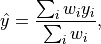
aperture. Optimal extraction refers to a weighted extraction designed to yield
the best signal-to-noise for background-limited targets (Naylor 1998). This page discusses
some details of the implementations and the advantages and disadvantages of
the various options, and summarises some other aspects of how things work.
Contents
Aperture positioning
A key problem faced by the pipeline is how to locate the targets from frame to
frame given that the telescope moves, and conditions vary. The usual option
in the reduce configuration file is the [apertures] section is
location = variable. It’s worth understanding how this operates. In the
usual case one defines one or more targets as reference apertures in
setaper. The aperture movement inside reduce then proceeds through a two
step process as follows:
First search for the first reference target in a box of half width
search_half_widtharound its last valid position. This search is carried out by smoothing the image (search_smooth_fwhm) and taking the location of whatever local maximum exceeds a pre-defined threshold (fit_height_min_ref) and lies closest to the last-measured position. The position of this maximum is used as the starting position for a 2D profile fit. This method is fairly robust against even bright cosmic rays as long as they lie further from the expected position than the target. The smoothing helps this as cosmic rays tend to be confined to 1 or 2 pixels. If reference targets are chosen to be bright and isolated, one can carry out broad searches which allow for very poor guiding. The shift measured from the first reference star is used to provide a better starting position for any remaining reference stars to improve things still more. This means that you should try to make the first reference star that appears in an aperture file for any given CCD the most robust of all. This is particularly the case if you have to makesearch_half_widthlarge because of bad guiding. Note that “robust” means unlikely to jumpt to another star so the key aspect is that it has no near stars of reference star type brightness. Following the search, 2D profile fits are carried out and the mean x,y shift relative to the starting position is calculated. If this stage fails (e.g. because of clouds), then the rest of the frame is skipped on the basis that if the reference targets cannot be located, then no others will be either. All the reference stars must be successfully relocated each time. This means an increased chance of failure compared to a single reference, but potentially can pay off in being more sensitive to problems: the parameterfit_diffis used for this by guarding against mutually discrepant reference positions. Again this acts in a severe all-or-nothing manner. The benefit is a lowered risk of losing the reference position altogether. If you find are losing the location of the stars on some frames then it is probably a case of adjusting the values ofsearch_half_width,search_smooth_fwhm,fit_height_min_refandfit_diff. ``Next, the positions of non-reference, non-linked apertures are determined. This is done through 2D profile fits starting from the shift determined from the reference targets. This allows a possibly wide-ranging initial search step as used for the reference stars to be skipped. The parameter
fit_max_shiftcan be used to control how far the profile fits are allowed to wander from the initial positions obtained via the reference stars. If the fits to non-reference stars fail, and there are reference stars available, an extraction will still be carried out. This allows one to cross over deep eclipses while still extracting flux at the known position offset of your target from the references.
The combination of the options available in setaper and the reduce
configuration file are a powerful means to track objects over many thousands of
exposures in a row. The main risk of failure comes when a combination of
clouds and cosmic rays cause a target to be too faint to register while a
cosmic ray does. Multiple reference stars and careful use of fit_max_shift
and fit_diff can help in such cases. A final option is fit_alpha which
enables averaging of the offset used to get from the reference stars to the
target position. This allows one to cope with, for example, stars that disappear
during eclipses, without simply fixing the offset in perpetuity using the link
option. fit_alpha = 0.01 for instance only applies a fraction of 0.01 of the
correction to the x,y offsets measured on a given frame. This has the effect of
smoothing the offsets over the scale of 100 frames or so. This should make the relative
aperture positions less jumpy than simply applying them directly. Experimentation is
advised to compare and optimise results. Once the aperture positions are
determined, reduce moves onto extracting the flux.
Target detection
The first stage of target detection is a search over a smoothed image. The
peak height thresholds fit_height_min_ref and fit_height_min_nrf are
important at this point. The effect of smoothing on a single pixel can be written as
where the  are the gaussian weights
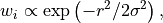
with  the distance in binned pixels from the particular pixel under
consideration, and
the distance in binned pixels from the particular pixel under
consideration, and  is the RMS of the smoothing being applied
(
is the RMS of the smoothing being applied
( ) and
) and  are the values
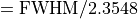
of the contributing surrounding pixels. A quantity of interest is the
statistical uncertainty of this smoothed value, since it is this which sets the
desirable threshold level. Assuming the contributing pixels are independent,
the variance is given by
are the values
of the contributing surrounding pixels. A quantity of interest is the
statistical uncertainty of this smoothed value, since it is this which sets the
desirable threshold level. Assuming the contributing pixels are independent,
the variance is given by
Assuming  , and that we are in a background-limited case
(which gives the minimum variance), the sums can be approximated as integrals
and one finds that
, and that we are in a background-limited case
(which gives the minimum variance), the sums can be approximated as integrals
and one finds that
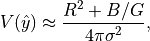
where  is the RMS readout noise in ADU,
  is the
background level in ADU and
is the
background level in ADU and  is the gain in electrons per ADU.
This relation fails when
is the gain in electrons per ADU.
This relation fails when  , so the denominator should
not go below this value (such a small smoothing would be an odd choice in any
case). An obvious threshold would be thus be some multiple of the equivalent
standard deviation
, so the denominator should
not go below this value (such a small smoothing would be an odd choice in any
case). An obvious threshold would be thus be some multiple of the equivalent
standard deviation
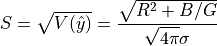
For example, assuming  ,
,  ,
,  and a smoothing FWHM of
10 leads to
and a smoothing FWHM of
10 leads to  . One would then expect to choose at least 3 times
this, and probably more because any given search area will include effectively
a number of “independent trials”, not just one, so the threshold will need
raising as a result. Choosing a lower threshold runs the risk of peaking up on
spurious noise peaks, especially when clouds are passing. This is not
desirable, particularly for reference targets. A target of seeing-limited peak
height
. One would then expect to choose at least 3 times
this, and probably more because any given search area will include effectively
a number of “independent trials”, not just one, so the threshold will need
raising as a result. Choosing a lower threshold runs the risk of peaking up on
spurious noise peaks, especially when clouds are passing. This is not
desirable, particularly for reference targets. A target of seeing-limited peak
height  in RMS seeing
  binned pixels will end up with
height
binned pixels will end up with
height
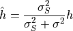
in the smoothed image, and thus the signal-to-noise of the smoothed peak will be
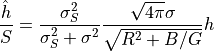
when we are background-limited (the case of most interest). This is maximised
by choosing  , so the smoothing FWHM ideally should match
the FWHM of the seeing (in terms of unbinned pixels). The smoothing is acting
as what is sometimes called a “matched filter”.
, so the smoothing FWHM ideally should match
the FWHM of the seeing (in terms of unbinned pixels). The smoothing is acting
as what is sometimes called a “matched filter”.
Warning
At the moment, the search routine uses fixed height thresholds; I expect to change them to depend upon the background level, so they will in future be specified as a multiplier of the above estimate.
Sky background estimation
The sky background is estimated from a circular annulus centred on each
target. The user can define the inner and outer radii. Inside setaper it is
possible to mask out obvious stars from the sky annulus for any target. To
some extent, the two methods implemented (median and clipped mean) should
eliminate contaminating stars, but they are not perfect and if you can see an
obvious star, it is best to mask it. You should, if possible, try to set the
sky annulus radii such that there is a much larger area of sky than in the
target aperture, i.e. 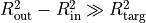 , in order to minimise the uncertainty due to the sky
estimate. The downside of this is the possibility of picking up more nearby
stars, starting to overlap the sky annulus with the edge of the window
within which the target falls, and increasing the size so much that
quadratic variations in the sky background become important. Overlap of the
sky aperture with the edge of the window is not desirable as one always wants
the sky to be symmetrical around the object to eliminate any gradients in the
sky.
, in order to minimise the uncertainty due to the sky
estimate. The downside of this is the possibility of picking up more nearby
stars, starting to overlap the sky annulus with the edge of the window
within which the target falls, and increasing the size so much that
quadratic variations in the sky background become important. Overlap of the
sky aperture with the edge of the window is not desirable as one always wants
the sky to be symmetrical around the object to eliminate any gradients in the
sky.
Normal extraction
As indicated above, normal extraction is essentially a case of adding all the pixels inside the inner circular aperture defining the target. It is not quite as simple as this because the pixels are square-shaped (or rectangular for non-equal binning factors) and not compatible with a circle, thus something needs to be done about the pixels at the edge. If they are simply included or excluded on the basis of how far their centres are from the centre of the target aperture, one can suffer from pixellation noise that occurs when pixels instantaneously appear or disappear owing to tiny change of target position. To reduce this I use the commonly-adopted soft-edge weighting scheme whereby a pixel which has its centre exactly on the edge of the circle gets a weight of 0.5, which is linearly ramped from 0 to 1 as the pixel approaches the aperture over a length scale comparable to its size.
An important element of normal extraction is the radius to extract the target flux from. In an ideal world with steady seeing, this would have a single value. However, seeing is very rarely steady, and can exhibit very variable behaviour in a night, or even within minutes. Thus a commonly used option is the ‘variable’ aperture option (set in the reduce file). This scales the radius of the extraction aperture to a multiple of the FWHM of the stellar profiles of the given frame. A single mean value of FWHM is established through profile fits to the targets and thus the same extraction radius is used for all targets. Useful values for the scale factor range from 1.5 to 2.5. Stellar profiles have extended wings, so one cane never include all the target flux in the aperture. Instead the hope is that the same fraction of flux is missed from both target and comparison, which then cancels when performing relative photometry. The exact choice of scale is not easy, as it represents a balance between increasing statistical noise for large radii versus increasing systematic noise for small radii when the fraction of flux lost from the apertures becomes large. Bright targets tend to push the choice towards large radii, while faint targets are better with small radii. The key is to try different values and compare the results side by side.
Sometimes one might have no suitable comparison star, or only ones of very different colour to the target such that they are bright in some bands but faint in others. If the weather is photometric, then extraction of just the target with a large aperture, reminiscent of the old days of photometry with photomultipliers through 10 or 15 arcsec diameter apertures, may be in order. It is also possible to use the comparison star on one band to correct for short timescale fluctuations in another where the comparison may be faint, but one should then typically use a larger than normal radius because the profiles of different bands are unlikely to be the same, and one also then needs to allow for differential atmospheric extinction over longer timescales.
A final rare possibility is to use a target as its own comparison. This can be useful if an object has very different behaviour at different wavelengths but no suitable comparison. A good example of this is the star V471 Tau which shows an eclipse of a white dwarf that is deep at short wavelengths but shallow at long wavelengths.
Profile fitting
In order to measure the FWHM to set the aperture size, HiPERCAM uses one of two possible forms of stellar profile, namely a 2D gaussian or “Moffat” profile, in each case symmetric. The gaussian profile is described by the following relation
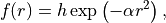
where is the distance from the centre of the gaussian, is
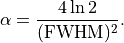
its height, and  is defined by the FWHM of the profile according
to
is defined by the FWHM of the profile according
to
Moffat profiles (Moffat 1969) usually provide much better fits to stellar profiles than gaussians. Moffat profiles are described by
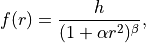
where now is a function of both the FWHM and  :
:
Moffat profiles tend to gaussians as  , anything
a gaussian can fit, they can. Their advantage is their more extended
wings which often give a better fit to real stellar profiles. However, they
also have a downside in that some profiles seem to fall off more steeply than
gaussians and when fitted with Moffat profiles, there is a tendency for the
value of to climb to very large values. This probably depends
upon the telescope and instrument, so should be the subject of
experimentation. In order to be integrable, they should have
, anything
a gaussian can fit, they can. Their advantage is their more extended
wings which often give a better fit to real stellar profiles. However, they
also have a downside in that some profiles seem to fall off more steeply than
gaussians and when fitted with Moffat profiles, there is a tendency for the
value of to climb to very large values. This probably depends
upon the telescope and instrument, so should be the subject of
experimentation. In order to be integrable, they should have  .
The profile fitting is implemented in
.
The profile fitting is implemented in hipercam.fitting on top of the
Levenberg-Marquardt fitting routine scipy.optimize.leastsq(). It is
designed to be able to sub-pixellate, i.e. the profile is evaluated at
multiple points within pixels to allow for cases where the seeing becomes
small compared to the pixels. This is controlled by the parameter fit_ndiv
in the reduce file. It’s use does come with a speed penalty owing to the
larger number of function evaluations.
Optimal photometry
For faint targets a significant improvement can be made by adding in the flux in a weighted manner, as discussed by Naylor (1998). As Naylor discusses, rather than the precisely “optimal weights” which are proportional to the expected fraction of target flux in a pixel divided by its variance, it is better in practice to use weights simply proportional to the expected fraction alone, as determined with some sort of profile fit. This is because this approach is robust to poor profile fits, which are not uncommon given the vagaries of seeing and guiding. This contrasts with the optimal extraction used in spectroscopy where the multiple pixels in the dispersion direction allow the development of good models of the spatial profile.
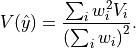
An example of the improvement possible with optimal photometry in shown in Fig. 4.
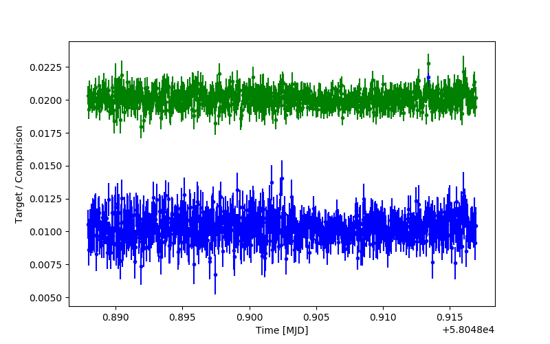
Fig. 4 Normal (blue) versus optimal (green) photometry of the same target relative to a much brighter comparison. The optimal photometry has been moved up by 0.01 for clarity.
In this case a faint target was chosen, and there is indeed an obvious improvement in signal-to-noise. The aperture radius in this case was set to 1.8 times the FWHM of the profiles, and, while a smaller size might yield a higher signal-to-noise for the normal photometry, one would not want to cut down very much because of loss of flux.
The choice of weights is designed so that one does not need the profile to be perfectly modelled, but it does require that both target and comparison have the same profile. If this is not the case, e.g. the CCDs have significant tilt leading to a FWHM that varies with position, then optimal photometry can suffer from systematic errors that make things worse. As usual, such problems manifest themselves most on bright targets, so one should not simply choose ‘optimal’ over ‘normal’ by default. (I use ‘normal’ most of the time.)