HiPERCAM Phase II

The most important part of the HiPERCAM phase II process is defining the finding chart and instrument setup in the tool hfinder. For HiPERCAM these two aspects are more tightly connected than is usually the case with CCDs, as will be described below. As a result perhaps, it is fairly common to see non-optimal phase II setups, so the aim of this page is to provide a blow-by-blow discussion of the series of considerations that you should go through to optimise your observations. The intention is that you work through these in series one by one, although you may also need to go back a step or two to iterate.

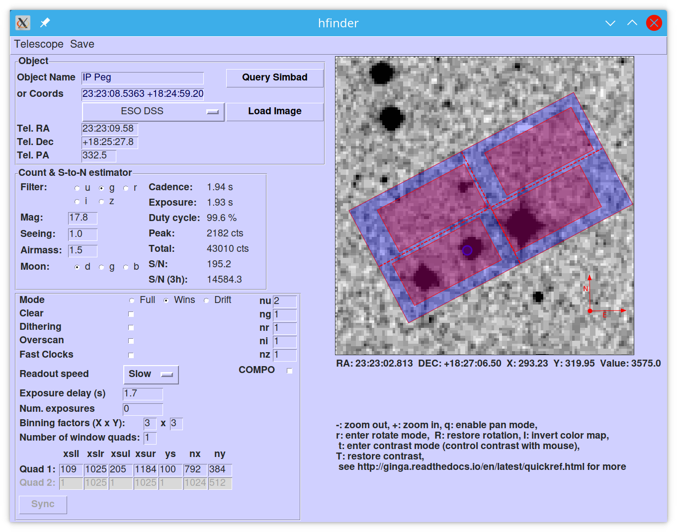
This is a fairly long document, but the considerations are somewhat involved, so please try to read it thoroughly. You are advised to read it in conjunction with running hfinder as it is referred to often, however in case you can’t for some reason here is a screen shot of hfinder in action:

If you are in a hurry, at least read through the various warnings as they might save you some future grief.

Checklist

To start off, here is a checklist for HiPERCAM’s phase II to prompt thought about your setup; the rest of the document expands on these items. The hope is that you have answers to all the questions!

1. What spatial sampling do you need? 1x1 binning is very rarely the best choice, and sometimes can have a very negative impact on noise. HiPERCAM’s native pixel size is only 0.081” on the GTC.

2. Could your setup lead to saturation in good seeing? If so, is there leeway for the observer to reduce the exposure time (a relatively easy change) without the need to change the setup (time consuming)?

3. Have you checked the peak counts per pixel in all CCDs, especially CCD 1 (u-band)? Is it comfortably above readout? (100 counts or more). The nskip parameters (nu, ng, nr, ni, nz) may help.

4. Is your target away from the medial lines of the CCDs in both X and Y to avoid a split readout and consequent data reduction problems?

5. Have you ensured that no very bright objects are aligned along the Y direction and in the same quadrant as your target?

6. For blue targets, have you included a bright comparison star (if available) for the u-band, even if it looks too bright for the griz bands?

7. For variable targets, have you considered the impact of the full range of their variability in terms of possible saturation or readnoise?

8. Is the duty cycle of your setup what you expect? For most observations it should be above 95%.

9. Is your setup tolerant of the full range of conditions you have specified for it? Variations in seeing especially, can cause dramatic variations in peak count levels and may veer you towards either saturation or readout noise limitations.

10. Does the product of the number of exposures and the cadence match the time you want to follow your target?

11. Do you need to dither your observations for optimum background subtraction?

Cadence / exposure time

The first thing you should decide is what cadence your science requires. The longer it is, the easier things tend to be. A key feature of HiPERCAM, if you are trying to go fast, is that there is a trade off between how fast you can go and how much of the CCDs you read out and/or what binning you use. If you try to go very fast, e.g. much less than a second, you will need to read sub-windows out, or bin the readout. For very fast observations there is a special option (“drift mode”) to reduce readout overheads further, and there are even observations too fast for drift mode where a special trick can be used at the expense of dead time overheads. Therefore, the exposure time can define multiple other aspects of the setup.

For any given setup (binning, window sizes, readout mode), there is an absolute minimum exposure time which is set by the time taken to readout the masked areas of the CCD. One can expose for longer than this minimum by adding an arbitrary “exposure delay”; this is a key parameter of the hfinder setup. So perhaps your setup can be readout in 3 seconds, but for reasons of signal-to-noise perhaps you add 7 seconds exposure delay. Then your exposure time (and cadence, as dead time is negligible in this case) will be 10 seconds. If you set the exposure delay to 0 however, your exposure will be 3 seconds and you wouldn’t be able to go faster without altering the setup. An important consideration in phase II is to avoid setups that make it likely that the observer is forced into changing the setup as this is costly in terms of time.

If your objects are not variable, then, as usual for CCD imaging, you should consider (a) the signal-to-noise you need, (b) the avoidance of saturation of your target and possibly comparison stars, (c) allowing enough time for the sky background to dominate over readout noise for faint sky-limited targets especially, and (d) whether you want to divide up exposures perhaps for dithering the position, or to enable exploitation of brief periods of best sky conditions, e.g. seeing.

For time-series observations of variable targets, considerations (a), (b) and (c) may still apply, but you also need to decide on the timescale you aim to sample. Because of the dependence of the minimum exposure time on the setup described earlier, this timescale may drive later decisions. For instance, HiPERCAM’s full frame, unbinned readout time is about 3 seconds. If you need to go faster than this, you will need to bin or window. This is a trivial but common example of the interplay between exposure time and CCD setup.

It is not unusual for the key driver of the exposure time to be the need to avoid saturation of the target and comparison stars. If this is the case, then you might need to allow yourself “headroom” when defining the setup in the sense that the observer has the possibility of reducing your exposure time without having to change setup, as described earlier.

Spatial sampling / binning

It is quite common to see setups with 1x1 binning selected. This may seem best in the sense of why would one want to degrade the best possible resolution? However, in very many cases 1x1 binning is not the optimal choice, and sometimes it is very much not the right choice. There are three reasons for this:

1. HiPERCAM’s native unbinned pixel size on the GTC is just 0.081 arcseconds, which significantly oversamples all but the very best seeing. Thus if you bin 2x2, 3x3 or even 4x4, you might not lose much resolution at all.

2. Binning substantially reduces the amount of data. This can allow you to readout the CCD faster. This could mean for example that you can read the entire CCD binned, whereas you would have to sub-window if unbinned. This can make observing easier, and ensure that objects are not too close to the edge of the readout windows.

3. Binning reduces the impact of readout noise. CCD binning occurs on chip before readout, so readout noise is incurred per binned pixel, not per native CCD pixel. This is often very important gain, depending upon target and sky brightness. You should, if possible, define a setup that ensures that the peak target counts per binned pixel are substantially in excess of where is the RMS readout noise in counts (ADU) and is the gain in electrons per ADU. For HiPERCAM this means one wants if possible at least 100 counts/pixel at peak, and preferably higher than this. There is a caveat to this in that if the sky counts are greater than this level, then there is less to be gained since binning increase the target and sky counts per pixel by the same factor, but when going fast, the sky can often be quite low level (especially in CCDs 1, 2 and 3, i.e. ugr). This means it can make sense sometimes to use very large binning factors when going fast and sky noise is low. It is this sort of case when binning can quite dramatically improve your data, and if you are not worried about spatial resolution at all, 8x8 or even 16x16 binning might make sense.

Binning has downsides of course; resolution is the obvious one. If you need to exploit good seeing, then you may not want to go beyond 2x2 binning. The other one is that you make saturation more likely of course. However, points 2 and 3 above mean that more often than not you should bin, and you should think twice before simply selecting 1x1. To understand more about how one guard against readout noise, see the section below on condition-tolerant setups.

Note

The binning is the same for all CCDs. There is another option for accounting for differences between CCDs. See the discussion of nskips below.

Note

The peak counts per binned pixel are displayed by hfinder if you set the correct magnitude for the target and selected filter. This is a very good way to judge your setup.

Full vs Wins vs Drift modes

hfinder includes buttons to select between various modes. “Full” reads the entire CCD (if the binning factors are compatible). “Wins” can also read the entire CCD, but allows one to define sub-windows (and in some cases is needed simply to get binning-compatible sizes, e.g. for 3x3 binning). After binning, defining sub-windows is the easiest way to speed up the readout.

In either full frame or windowed mode, at the end of each exposure, the entire imaging portion of the CCD (including pixels that won’t be saved) is moved into the masked area prior to readout. This involves a charger transfer in the Y-direction of half the frame height, which costs some deadtime. In very high-speed cases, this overhead can rise to unacceptable levels. The way to reveal this is to switch to windowed mode, choose some fairly high binning, a minimal exposure delay, and then start to chop the windows down. As one does so, the reported “Duty cycle” starts to drop below 100%, as the result of the frame transfer overhead. e.g. with 8x8 binning and 128x128 windows, the cadence is around 0.017 seconds, the actual exposure per frame 0.0092 seconds and the duty cycle is around 50%. “Drift” mode is designed to reduce the overheads through partial frame transfers. In this case, the cadence (exposure) times become 0.0137 (0.0118) secs for an 86% duty cycle. Dropping to 128x64, delivers a cadence of 0.0069 secs at 86% in drift, cf 0.0124 at 37% in windowed mode, so for efficient observations faster than a few 10s of Hertz, drift mode can offers significant efficiency gains.

nskips

When running hfinder you will see a series of integers arranged in a column and labelled nu, nu, nr, ni, nz, and set by default to 1, 1, 1, 1, 1. These are the “nskip” parameters which dictate how often each CCD is readout. The chief purpose of these is to compensate for the often significant variations of count rates between the CCDs. Thus consider a target of magnitude g=20, u=20. In one second, and 4x4 binning, hfinder reports 262 counts at peak in g, but only 40 in u, so the u band is below the readout threshold discussed earlier. If one is happy instead to use 3 second exposures in u, then this can be fixed by setting nu = 3.

Warning

The peak counts reported by hfinder do not account for the nskip values, so you need to take them into account when judging the peak count level. You should check values for all CCDs.

Note

It is usual to run with at least one of the nskip values set = 1, so that at least one CCD is read out every time. One could in principle set values like 5,4,3,2,2,3 to deliver fractional exposure time ratios. It is not advises though, because (i) there should be enough dynamic range between readout-limited data and saturated data that integer ratios are OK, (ii) each CCD is always readout each cycle, but nskip-1 of the readouts are dummy readouts producing junk data. Thus with a minimum nskip of 2, at least 50% of the data for each CCD is junk. The software is designed to ignore this, but it is wasteful of disk space. A set of nskip values like 9,6,3,3,3 i.e. with a common divisor, is a mistake as it could be changed to 3,2,1,1,1 and the exposure delay adjusted to triple the cadence. This would deliver identical data but cut down the overall size by a factor of 3.

Comparison stars

If you have to use windows, their exact definition very much depends upon the field of your target. At minimum one should include at least one and preferably two or more comparison stars if possible. They should be brighter than your target. It often helps to have one that is quite significantly brighter for the u-band, particularly for blue targets, as the average comparison is red, and it can quite often be the case that a comparison that is moderately brighter than the target in the redder bands is scarcely visible in u. Remember one does not need to use the same star as comparison in each filter and its OK for a comparison used in u to saturate in all other bands, as long as there is a backup comparison for those bands.

Warning

Avoid setups in which a bright star is on the same column (i.e. same X position) and same quadrant as a faint target. This is because the frame transfer leaves a low level vertical streak that could be problematic if there is a very bright star lined up with your target.

Warning

Do not place your target or comparisons close to the half-way point in either X or Y in full frame mode because the HiPERCAM CCDs are read out at the 4 corners and you risk your target being divided across multiple outputs.

Condition-tolerant setups

If you are sure that your target will only observed with seeing close to 1.2” and during clear conditions, you’ll have a relatively easy job defining a setup. Much more difficult is if the seeing could be anything from 1.2 to 2.5”, the reason being that the peak counts could vary by more than a factor of 4. The key point here is probably the binning. It should definitely be at least 4x4, and arguably 6x6 to 8x8, otherwise you could end up swamping the target with readout noise during poor seeing. One way to think about readout noise is as the equivalent of counts from the sky in each binned pixel. If you use 1x1 rather than 8x8, you have just increased this contribution by a factor of 64. Sometimes this won’t matter; sometimes it will be a disaster. As always, the thing to do is try different setups and seeing values in hfinder, and the key to using it is to understand the signal-to-noise values hfinder reports.

S/N vs S/N (3h)

If you look at hfinder you will see two values of signal-to-noise. One, “S/N”, is the signal-to-noise of one frame. The other, “S/N (3h)”, is the total signal-to-noise after 3 hours of data. The latter can reach unrealistically large values (e.g. 14584 in the screenshot) which are meaninglessly high in practice, nevertheless, the “S/N (3h)” value is one of the best ways to compare different setups as it accounts for the issue of shorter exposures versus a larger number of exposure and also deadtime. One way to find a condition tolerant setup is to find one where the “S/N (3h)” value does not respond dramatically to the exact setup.

As an example, consider a star of g=18 being observed at high speed in dark time, seeing 1”, airmass 1.5. With 1x1 binning and windows of 92x92, I find a cadence of 0.101, a duty cycle of 92.3% and an “S/N (3h)” value of 3772. This is not obviously bad, but the peak counts are listed as just 10! This will be heavily read noise affected. This becomes obvious if I add 0.1 seconds to the exposure delay giving 0.201 cadence, 96.1% duty. The S/N (3h) becomes 5306. That’s the equivalent of 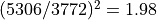times longer exposure, but the duty cycle only increased by a factor of 1.04. The large improvement is because I have halved the number of readouts.

What if I still want the 0.1 seconds? Then I should bin. So, the same target and conditions, but now with binning 4x4 and cadence 0.1 seconds, I find again a 92% cadence, but the S/N (3h) value is now 9970 and I have gained a factor of 7 in effective exposure time! So the first setting was really a disaster. To judge how much further there is to go, I make the cadence 10 sec, and find S/N (3h) = 13400, but of course 10 seconds may be unacceptably long, but still it shows what one should be aiming at.

What about the impact of seeing? If I set seeing to 2”, the S/N (3h) for the 4x4, 0.1-sec mode drops to 6265, equivalent to dropping the exposure down by a factor 0.4. The 1x1 version drops to 1937, equivalent to just 0.26 of the exposure, so not only is it a bad setup, but it gets worse more quickly.

Warning

These are not small effects, and you need to think about them for all CCDs. CCD 1 (the u-band) is almost always the most sensitive of all to readout noise issues. “nskip” is your friend then. If possible try to find the sweet spot between being well above the readout noise, but not in danger of saturation. Peak counts (factoring in any nskips) from 1000 to 15000 are what you might want to aim for, although they won’t always be possible.

Beyond drift mode

If you want to go fast, you will probably need to window, and as pointed out above, if you want to really fast, drift mode can be useful. If you want to go really fast, and can take a hit in terms of efficiency, then windows plus “clear” might be what you want. This is because you can expose for just the exposure delay by clearing the CCD immediately before starting the exposure. With clear enabled, the exposure time just equals the exposure delay, with no added extra for the readout of the masked data. e.g.